Friday March 29 CSL Meeting

2019 Annual AAG Meeting Preview

Presenters: Bradley Barger, Nicole Casamassina, Victoria Ford
Time: Friday, 29 March 2019, 2:00-3:00 p.m.
Location: 805 O&M

Local and Remote Drivers of Cyclones in Baffin Bay & Davis Strait

Bradley Barger

Abstract: Cyclones are a primary mode of energy transport in the Arctic. Connected to the planetary atmospheric flow and influenced by local and remote fluctuations in pressure and temperature, cyclones range in strength, duration, and location throughout the year. In the North Atlantic region, the mechanisms that cause cyclogenesis, deepening, and cyclolysis are well documented. However, the effects of local and remote drivers on cyclone frequency and migration need to be further investigated. Previous studies have shown that North Atlantic cyclones are impacted by Greenland and bifurcate at its southern tip. However, no studies have investigated what happens to the portions of the bifurcated cyclones once they enter the Davis Strait. This project analyzes the effects of sea ice cover and major atmospheric teleconnections on cyclone frequency and migration in the Baffin Bay/Davis Strait region of the Arctic from 1980-2015. Monthly sea ice data were provided by the National Snow and Ice Data Center; monthly teleconnection indices were provided by the NOAA Climate Prediction Center and National Centers for Environmental Information; and daily cyclone data were obtained from the Goddard Institute for Space Studies at NASA. Analysis of sea ice data and teleconnection indices suggest that cyclones and sea ice extent respond to fluctuations in certain teleconnection patterns, while other teleconnections cause little to no effect. In addition, the cyclone frequency observed in the Baffin Bay/Davis Strait region are highly variable at different timescales. In the future, local cyclone trends could possibly be used to indicate climate change in this region.

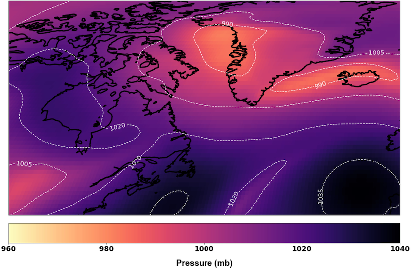Cyclone bifurcation due to colliding with Greenland's southern tip. One system tracks into Baffin Bay while the other continues into the North Atlantic.

Estimating Losses from Hurricane Harvey Using FEMA's HAZUS-MH Model

Nicole Casamassina

Abstract: Hurricane Harvey was one of the most destructive and costliest hurricanes to ever make landfall on the Texas coast and one of the many tropical cyclones that impacted the United States during the 2017 North Atlantic Hurricane Season. In recent years, emergency managers and researchers have been using hurricane risk and vulnerability analyses developed through the use of Geographic Information Systems (GIS) to make informed decisions on different aspects of community and regional preparedness when a tropical cyclone is forecasted to impact an area. Though there are many ways to quantify risk and vulnerability, this project uses the Federal Emergency Management Agency's (FEMA) Hazards-US Multi-Hazards (HAZUS) GIS extension to estimate and illustrate the physical, economic, and social losses associated with tropical cyclone impacts along the Texas coast. There are numerous ways to quantify the risks associated with tropical cyclones using GIS, most of which focus on one of the three hazards involved in hurricane impact: extreme winds, heavy rainfall, and storm surge. This project addresses this shortcoming by focusing on all three hazards and modelling the physical, economic, and social losses in locations in Texas that were caused by Hurricane Harvey. Heavy rainfall produced the most losses, while storm surge affected the southern-most areas of the Texas coast. Wind damage was most prominent near Rockport, TX, where winds were estimated around 130 mph. The results of this study are compared to risk analyses developed by government agencies to seek way to improve current mitigation strategies in the region.

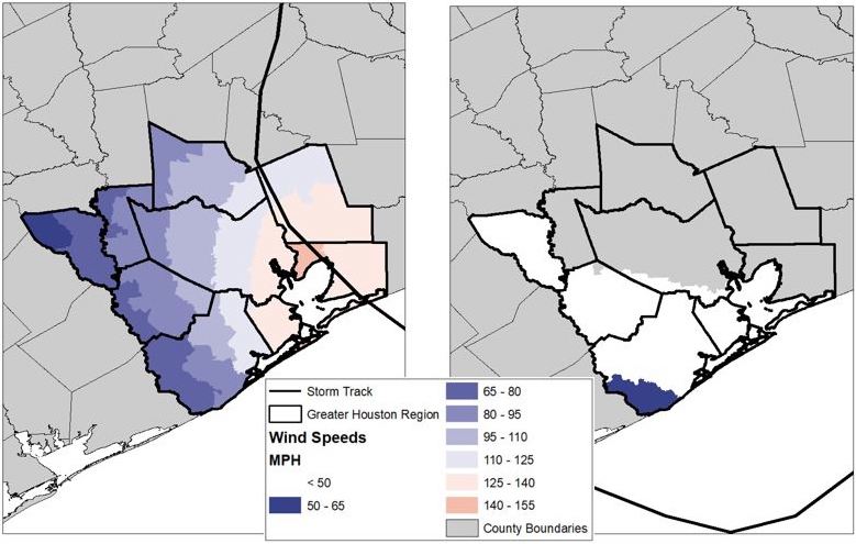Estimated wind speeds and storm tracks for a probabilistic 200-year return period hurricane and Hurricane Harvey in the Greater Houston Region.

The Influence of Arctic Sea Ice Thinning on the Atmospheric Boundary Layer

Victoria Ford

Abstract: As one of the most visible indicators of a warming climate, the Arctic sea ice cover has been experiencing a transition from thick, multiyear ice into much thinner, first-year ice. This transition has been observed in sea ice extent and thickness, with variations at different spatial scales. Energy exchange between the Arctic Ocean and atmosphere, through the sea ice pack, is expected to increase with a thinner overlying ice cover, which typically acts as an insulator from the relatively warm Arctic Ocean. Open water heat fluxes exhibit the greatest response in the Arctic atmospheric boundary layer, while thick ice presence results in minimal heat conduction. Polar-optimized Weather Research and Forecasting model simulations assess how a wintertime Arctic boundary layer responds to sea ice thinning via the associated increase in surface air temperature and sensible heat flux exchange. This thermodynamic response increases as sea ice thickness is simulated transitioning from perennial to seasonal ice. Sea ice thicknesses less than 1 meter are sufficient in heating the surface boundary layer in winter despite ice presence. Accurate wintertime sea ice thickness estimates have been shown to determine sea ice coverage in subsequent seasons, thus motivating timely and precise future sea ice thickness prediction in the transitioning seasonal ice regions.

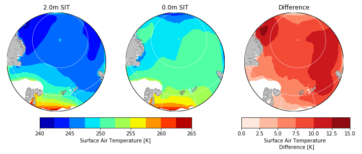Arctic surface air temperature patterns over idealized uniform ice thicknesses in January 2000. Left: two meter thick sea ice thickness; middle: zero meter sea ice thickness; right: difference between middle and left plots, highlighting increase in temperature with sea ice thickness reductions.